import pandas as pd
import numpy as np
import matplotlib.pyplot as plt

import holoviews as hv
hv.extension('bokeh')

from tqdm.notebook import tqdm

The Imputation Problem¶

df = pd.read_csv('dataset.csv', parse_dates=True, index_col=0)
df.columns = ['S_' + n for n in df.columns] # some packages get confused with integers as column names. Use alphanumeric column names

Here is a dataset with missing values.

df.head(10)

plt.imshow(df.T, aspect='auto', interpolation='nearest')
plt.xlabel('Time')
plt.ylabel('Station')

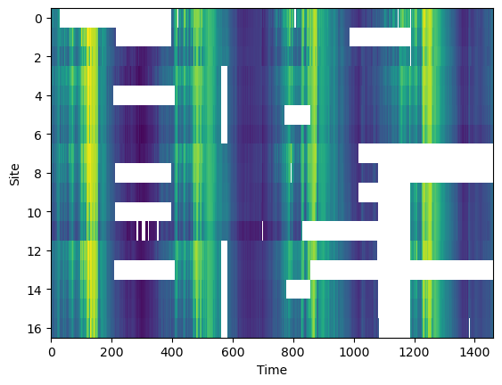
We wish to examine different imputation algorithms to see how they compare with each other. In this study we consider KNN, MICE, MissForest, and a simple linear univariate method. The process is adaptable to other imputation based methods.

def missing_data_fraction(df):
    X = df.values
    N = X.size
    m = np.isnan(X).sum()
    missing_data = m / N * 100
    return missing_data

print (f'Original missing data {missing_data_fraction(df):0.1f}%')

Original missing data 14.8%

With a signifcant amount of missing data, it is impossible to evaluate how well the imputation algorithm is doing. We need to know the true values that the algorithms are trying to estimate.

We take our dataset at restrict it the study sites where at least 90% of the data is available. Once we have validated that the imputation algorithm are working as expected we will come back and use the best one to fill in more of the missing data in the dataset.

# Calculate the percentage of non-missing data for each study site
non_missing_percentage = df.notna().mean() * 100

# Filter study sites with at least 90% non-missing data
selected_sites = non_missing_percentage[non_missing_percentage >= 99].index
df_selected = df[selected_sites]

plt.imshow(df_selected.T, aspect='auto', interpolation='nearest')
plt.xlabel('Time')
plt.ylabel('Station')

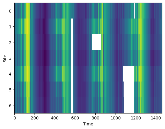
print (f'Missing data {missing_data_fraction(df_selected):0.1f}% for "ground truth"')

Missing data 0.3% for "ground truth"

We will refer to this dataset as the true dataset for comparison to the estimated reconstructions. Notice that even this dataset has some missing data.

df_true = df_selected.copy()

Introduce artifical gaps¶

Prepare the dataset by introducing artificial gaps. We can randomly select a fixed number of sites and introduce gaps of a fixed length.

def add_artificial_gaps(df, num_sites=24, gap_length=56):
    np.random.seed(4152)

    gaps = {}
    # randomly set a n-day contiguous segment as missing for each column
    random_columns = np.random.choice(df.columns, size=num_sites, replace=False)
    
    N = len(df.values.flatten())
    m = df.isnull().values.flatten().sum()
    missing_data = m / N * 100
    
    for col in random_columns:
        # Randomly select the start of the n-day segment
        start_idx = np.random.randint(0, len(df) - gap_length)
        end_idx = start_idx + gap_length
    
        gaps[col] = [start_idx, end_idx]
    
        # Set the values in this range to NaN
        df.iloc[start_idx:end_idx, df.columns.get_loc(col)] = np.nan

df = df_true.copy()
add_artificial_gaps(df, 16, 30)

plt.imshow(df.T, aspect='auto', interpolation='nearest')
plt.xlabel('Time')
plt.ylabel('Station')

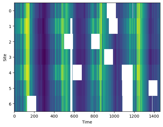
print (f'Artificial missing data {missing_data_fraction(df):0.1f}%')

Artificial missing data 1.6%

We can vary the parameters of the number of sites and gap length to explore how the different imputation algorithms perform with different about of missing data.

Evaluation¶

Scikit-Learn has a general approach to using imputation algorithms that we mirror here.

from sklearn.impute import SimpleImputer

imputer = SimpleImputer(missing_values=np.nan, strategy='mean')

# Fit and transform the dataset
df_imputed = pd.DataFrame(imputer.fit_transform(df), columns=df.columns, index=df.index)

Replace with interactive visualization

dictionary = { int(i[2:]): hv.Overlay( [
    hv.Curve(df_true[str(i)], label='Truth'),
    hv.Curve(df_imputed[str(i)], label='Imputed'),
    hv.Curve(df[str(i)], label='Artificial Gap'),
]) for i in df_true.columns} 
hv.HoloMap(dictionary, kdims='Study Site').opts(aspect=2, title='Simple Imputer (mean)')

To evaluate this fit we compare back with the truth. We can calculate the Mean Absolute Error and the Root Mean Square Error.

error = df_imputed - df_true

MAE = np.mean(abs(error))
RMSE = np.sqrt(np.mean((error)**2))

print(f'MAE = {MAE:.2f}, RMSE = {RMSE:.2f}')

MAE = 0.02, RMSE = 0.39

We will compare different methods in terms of these metrics and as function of the relative fraction of missing data.

Imputation methods¶

Linear interpolation¶

This is a univariate method where we infill the missing data with a straight line between boundary points on any interval.

df_imputed = df.interpolate(method='linear')

dictionary = { int(i[2:]): hv.Overlay( [
    hv.Curve(df_true[str(i)], label='Truth'),
    hv.Curve(df_imputed[str(i)], label='Imputed'),
    hv.Curve(df[str(i)], label='Artificial Gap'),
]) for i in df_true.columns} 
hv.HoloMap(dictionary, kdims='Study Site').opts(aspect=2, title='Linear Interpolation')

error = df_imputed - df_true

MAE = np.mean(abs(error))
RMSE = np.sqrt(np.mean((error)**2))

print(f'MAE = {MAE:.2f}, RMSE = {RMSE:.2f}')

MAE = 0.01, RMSE = 0.10

MissForest¶

This is a reimplementation in Python of the algorithm from the original paper which in turn wraps the random forest regressor from scikit-learn. There are other MissForest implementations available in PyPi but I was not able to get them to be successful.

from sklearn.ensemble import RandomForestRegressor

def imputeMF(X, max_iter=10):

    mask = np.isnan(X)

    # Count missing per column
    col_missing_count = mask.sum(axis=0)
    
    # Get col and row indices for missing
    missing_rows, missing_cols = np.where(mask)

    Ximp = X.copy()

    # 1. Make initial guess for missing values
    col_means = np.nanmean(X, axis=0)
    Ximp[missing_rows, missing_cols] = np.take(col_means, missing_cols)

    # 2. misscount_idx: sorted indices of cols in X based on missing count
    misscount_idx = np.argsort(col_missing_count)

    iter_count = 0
    gamma_new = 0
    gamma_old = np.inf

    col_index = np.arange(Ximp.shape[1])

    rf_regressor = RandomForestRegressor(n_jobs=-1)

    while(gamma_new < gamma_old and iter_count < max_iter):
        
        #4. store previously imputed matrix
        Ximp_old = np.copy(Ximp)
        
        if iter_count != 0:
            gamma_old = gamma_new
            
        #5. loop for s in k
        for s in tqdm(misscount_idx):
            # Column indices other than the one being imputed
            s_prime = np.delete(col_index, s)
        
            # Get indices of rows where 's' is observed and missing
            obs_rows = np.where(~mask[:, s])[0]
            mis_rows = np.where(mask[:, s])[0]
        
            # If no missing, then skip
            if len(mis_rows) == 0:
                continue
        
            # Get observed values of 's'
            yobs = Ximp[obs_rows, s]
        
            # Get 'X' for both observed and missing 's' column
            xobs = Ximp[np.ix_(obs_rows, s_prime)]
            xmis = Ximp[np.ix_(mis_rows, s_prime)]
        
            # 6. Fit a random forest over observed and predict the missing
            rf_regressor.fit(X=xobs, y=yobs)
            
            # 7. predict ymis(s) using xmis(x)
            ymis = rf_regressor.predict(xmis)
            
            # 8. update imputed matrix using predicted matrix ymis(s)
            Ximp[mis_rows, s] = ymis
        
        # 9. Update gamma (stopping criterion)
        gamma_new = np.sum((Ximp - Ximp_old) ** 2) / np.sum(Ximp ** 2)
        iter_count += 1
    
        print('Statistics:')
        print(f'iteration {iter_count}, gamma = {gamma_new}')

    return Ximp

MissForest is a non-parametric method but we can set a maximum number of iterations.

df_imputed = pd.DataFrame(imputeMF(df.values, 3), columns=df.columns, index=df.index)

dictionary = { int(i[2:]): hv.Overlay( [
    hv.Curve(df_true[str(i)], label='Truth'),
    hv.Curve(df_imputed[str(i)], label='Imputed'),
    hv.Curve(df[str(i)], label='Artificial Gap'),
]) for i in df_true.columns} 
hv.HoloMap(dictionary, kdims='Study Site').opts(aspect=2, title='MissForest')

error = df_imputed - df_true

MAE = np.mean(abs(error))
RMSE = np.sqrt(np.mean((error)**2))

print(f'MAE = {MAE:.2f}, RMSE = {RMSE:.2f}')

MAE = 0.00, RMSE = 0.04

KNN¶

For K Nearest Neighbours (KNN), a hyperparameter is the number of neighbour to use. We will tune this hyperparameter.

from sklearn.impute import KNNImputer

imputer = KNNImputer(n_neighbors=7)

df_imputed = pd.DataFrame(imputer.fit_transform(df), columns=df.columns, index=df.index)

dictionary = { int(i[2:]): hv.Overlay( [
    hv.Curve(df_true[str(i)], label='Truth'),
    hv.Curve(df_imputed[str(i)], label='Imputed'),
    hv.Curve(df[str(i)], label='Artificial Gap'),
]) for i in df_true.columns} 
hv.HoloMap(dictionary, kdims='Study Site').opts(aspect=2, title='KNN')

error = df_imputed - df_true

MAE = np.mean(abs(error))
RMSE = np.sqrt(np.mean((error)**2))

print(f'MAE = {MAE:.2f}, RMSE = {RMSE:.2f}')

MAE = 0.00, RMSE = 0.06

MICE¶

from statsmodels.imputation.mice import MICEData

mice_data = MICEData(df, k_pmm=1)
n_iterations = 10
mice_data.update_all(n_iterations)

df_imputed = pd.DataFrame(mice_data.data.values, columns=df.columns, index=df.index)

df_imputed

dictionary = { int(i[2:]): hv.Overlay( [
    hv.Curve(df_true[str(i)], label='Truth'),
    hv.Curve(df_imputed[str(i)], label='Imputed'),
    hv.Curve(df[str(i)], label='Artificial Gap'),
]) for i in df_true.columns} 
hv.HoloMap(dictionary, kdims='Study Site').opts(aspect=2, title='MICE')

error = df_imputed - df_true

MAE = np.mean(abs(error))
RMSE = np.sqrt(np.mean((error)**2))

print(f'MAE = {MAE:.2f}, RMSE = {RMSE:.2f}')

MAE = 0.01, RMSE = 0.10

MissForest implementation¶

Identify missing observations

mask = np.isnan(df)

plt.imshow(mask, aspect='auto', interpolation='nearest')
plt.xlabel('s')
plt.ylabel('i')
plt.show()

# Count missing per column
col_missing_count = mask.sum(axis=0)

# Get col and row indices for missing
missing_rows, missing_cols = np.where(mask)

Ximp = X.copy()

# 1. Make initial guess for missing values
col_means = np.nanmean(X, axis=0)
Ximp[missing_rows, missing_cols] = np.take(col_means, missing_cols)

error = Xtrue - Ximp
MAE = np.nanmean(abs(error))
RMSE = np.sqrt(np.nanmean((error)**2))
print(MAE, RMSE)

0.06982506172103002 0.682397283867648

# 2. misscount_idx: sorted indices of cols in X based on missing count
misscount_idx = np.argsort(col_missing_count) # k

Stop when difference between the newly imputed data matrix and the previous one increases for the first time

iter_count = 0
gamma_new = 0
gamma_old = np.inf

col_index = np.arange(Ximp.shape[1])

from sklearn.ensemble import RandomForestRegressor
rf_regressor = RandomForestRegressor(n_jobs=-1)

from tqdm.notebook import tqdm

while(gamma_new < gamma_old):
    
    #4. store previously imputed matrix
    Ximp_old = np.copy(Ximp)
    
    if iter_count != 0:
        gamma_old = gamma_new
        
    #5. loop for s in k
    for s in tqdm(misscount_idx):
        # Column indices other than the one being imputed
        s_prime = np.delete(col_index, s)
    
        # Get indices of rows where 's' is observed and missing
        obs_rows = np.where(~mask[:, s])[0]
        mis_rows = np.where(mask[:, s])[0]
    
        # If no missing, then skip
        if len(mis_rows) == 0:
            continue
    
        # Get observed values of 's'
        yobs = Ximp[obs_rows, s]
    
        # Get 'X' for both observed and missing 's' column
        xobs = Ximp[np.ix_(obs_rows, s_prime)]
        xmis = Ximp[np.ix_(mis_rows, s_prime)]
    
        # 6. Fit a random forest over observed and predict the missing
        rf_regressor.fit(X=xobs, y=yobs)
        
        # 7. predict ymis(s) using xmis(x)
        ymis = rf_regressor.predict(xmis)
        
        # 8. update imputed matrix using predicted matrix ymis(s)
        Ximp[mis_rows, s] = ymis
    
    # 9. Update gamma (stopping criterion)
    gamma_new = np.sum((Ximp - Ximp_old) ** 2) / np.sum(Ximp ** 2)
    iter_count += 1

    error = Xtrue - Ximp
    MAE = np.nanmean(abs(error))
    RMSE = np.sqrt(np.nanmean((error)**2))

    print('Statistics:')
    print(f'iteration {iter_count}')
    print(f'gamma = {gamma_new}')
    print(f'MAE = {MAE:.3f}, RMSE = {RMSE:.3f}')

plt.imshow(Ximp, aspect='auto', interpolation='nearest')
plt.xlabel('s')
plt.ylabel('i')

Time Series Imputation for Oceanographic Data

Imputation

Time Series Imputation for Oceanographic Data

Determine hyperparameter n for KNN