Combine Time Series and Downsample - Time Series Imputation for Oceanographic Data

import pandas as pd
import os
import csv
import io
import numpy as np
import matplotlib.pyplot as plt
from tqdm.notebook import tqdm

We have distinct segments of sensor data.

metadata = pd.read_csv('metadata.csv')
metadata

Sensor are deployed many different depths in the water column

metadata['depth (m)'].unique()

array([ 2.  ,  6.  ,  4.  ,  1.  ,  1.3 ,  0.5 ,  1.5 ,  0.4 ,  0.8 ,
        1.6 , 16.  , 15.  , 14.  ,  0.  ,  5.  ,  7.  , 30.  , 18.  ,
       10.  , 20.  ,  3.  ,  3.5 ,  0.41, 26.  , 25.  , 75.  , 40.  ,
       50.  , 22.  , 28.  , 36.  ,  9.  , 60.  , 44.  , 24.  , 27.  ,
       12.  , 21.  , 16.5 ,  8.  , 17.5 , 37.  , 11.  , 13.  ,  4.5 ])

But most often, there are standard depths that are most often used:

metadata['depth (m)'].value_counts().head(15)

depth (m)
2.0     195
5.0     184
10.0    156
15.0    132
20.0     93
1.0      50
30.0     35
25.0     25
0.5      18
40.0     16
4.0      14
3.0      13
1.5      10
8.0      10
27.0     10
Name: count, dtype: int64

Let’s group these observation segments into more limited number of study sites where the waterbody, station, and depth are the same even if the sensor itself is replaced.

depths_list = [2.0, 5.0, 10.0, 15.0, 20.0]
study_sites = metadata[metadata['depth (m)'].isin(depths_list)][['waterbody', 'station', 'depth (m)']].drop_duplicates()
study_sites.reset_index(drop=True, inplace=True)

study_sites

For any of these study sites we can consider all of the observational segements at that station and depth.

study_site = study_sites.iloc[37]

subset = metadata[ (metadata['waterbody'] == study_site['waterbody']) &  (metadata['station'] == study_site['station']) & (metadata['depth (m)'] == study_site['depth (m)'])]
display(subset)

fig, ax = plt.subplots(2,1, figsize=(12,6),sharex=True)

variable = 'temperature (degrees_Celsius)'
qc_flag = 'qc_flag_temperature'

series_segments = []
for index, row in subset.iterrows():

    csvfile = f"segments/{row['segment']}.csv"
       
    series = pd.read_csv(csvfile, index_col='time (UTC)', parse_dates=True)
    series.sort_index(inplace=True)

    # blank out observations that do not pass QC
    series[series[qc_flag] != 'Pass'] = np.nan
    series = series.drop(columns=[qc_flag])
    
    ax[0].plot(series.index, series[variable])
    
    ax[0].set_ylabel(variable)
    ax[0].set_title(f'{study_site.waterbody}:{study_site.station} at {study_site['depth (m)']} m')

    if series.count()[variable] > 0:
        series_segments.append(series)

series_df = pd.concat(series_segments)
series_df.sort_index(inplace=True)

ax[1].set_title('Resampled to daily mean')
daily_series_df = series_df.resample('D').min()
ax[1].plot(daily_series_df.index, daily_series_df[variable], label='min', linewidth=0.5)
daily_series_df = series_df.resample('D').max()
ax[1].plot(daily_series_df.index, daily_series_df[variable], label='max', linewidth=0.5)
daily_series_df = series_df.resample('D').mean()
ax[1].plot(daily_series_df.index, daily_series_df[variable], label='mean')

ax[1].set_ylabel(variable)

At the time scale of four years, daily means are sufficient to see the cycle. The plot above shows the daily minimum and daily maximum.

Combine segments into time series¶

We aggregate together these different segments from different deployments (and possibly different sensor) to create a complete daily time series at each station and depth in our study area:

start_date = "2020-09-01"
end_date = "2024-08-31"

daily_time_index = pd.date_range(start=start_date, end=end_date, freq='D')

all_timeseries = []

for study_site_id in tqdm(study_sites.index):

    study_site = study_sites.iloc[study_site_id]
    #print(f'[{study_site_id}] {study_site.waterbody}:{study_site.station} at {study_site['depth (m)']} m')
    study_site_name = f'{study_site.waterbody.replace(' ','')}_{study_site.station.replace(' ','')}_{study_site['depth (m)']:.0f}'
    
    subset = metadata[ (metadata['waterbody'] == study_site['waterbody']) &  (metadata['station'] == study_site['station']) & (metadata['depth (m)'] == study_site['depth (m)'])].copy()
    
    segments = []
    for segment_id, row in subset.iterrows():

        csvfile = f"segments/{row['segment']}.csv"
        segment = pd.read_csv(csvfile, index_col='time (UTC)', parse_dates=True)
        
        segment.sort_index(inplace=True)

        # blank out observations that do not pass QC
        segment[segment[qc_flag] != 'Pass'] = np.nan
        segment = segment.drop(columns=[qc_flag])

        if segment.count()[variable] > 0:
            segments.append(segment)

    if len(segments) > 0:
        
        timeseries = pd.concat(segments)
        timeseries.columns = [study_site_id]
        
        timeseries.sort_index(inplace=True)

        daily_timeseries = timeseries.resample('D').mean()

        all_timeseries.append(daily_timeseries)

dataset = pd.concat(all_timeseries, axis=1)

This is our temperature dataset. It also define the starting point for reproducing this analysis with a different data set. We have measurements on same time resolution for many different measurements. Each column in the dataset represents a different measurement. We use NaN to represent daily measurements that are missing.

The goal of imputation is to make a good estimate of what values to replace those NaN that, while still an estimate, are justifiable.

dataset

Missing Data¶

How much of this dataset is actually missing?

non_missing_data = ~dataset.isna()

import seaborn as sns
from matplotlib.dates import DateFormatter

plt.figure()
sns.heatmap(non_missing_data.T, xticklabels= 180, cmap=['white', 'black'], cbar=False)

plt.ylabel('Study Site ID')
plt.title(f'Presence of measurement over time')

# Rotating the time axis labels for better readability
plt.xticks(rotation=45, ha='right')

plt.show()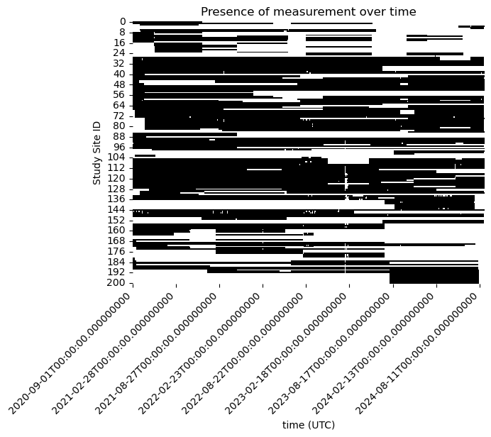

Some of our study site have very limited measurements at any time. We focus the problem more narrowly and ask what is the best estimate of the missing data when there is at least 50% of the observations available at a study site.

# Calculate the percentage of non-missing data for each study site
non_missing_percentage = dataset.notna().mean() * 100

# Filter study sites with at least 50% non-missing data
selected_sites = non_missing_percentage[non_missing_percentage >= 50].index
df_selected = dataset[selected_sites]

# Creating a boolean DataFrame where True indicates non-missing data
non_missing_data = ~df_selected.isna()

# Plotting
plt.figure(figsize=(12, 8))
sns.heatmap(non_missing_data.T, xticklabels= 180, cmap=['white', 'black'], cbar=False)

# Formatting the time axis labels
date_format = DateFormatter('%Y-%m-%d %H:%M')
#plt.gca().xaxis.set_major_formatter(date_format)

plt.xlabel('Time')
plt.ylabel('Study Site ID')
plt.title(f'Presence of {variable} Over Time (> 50%)')

# Rotating the time axis labels for better readability
plt.xticks(rotation=45, ha='right')
plt.show()

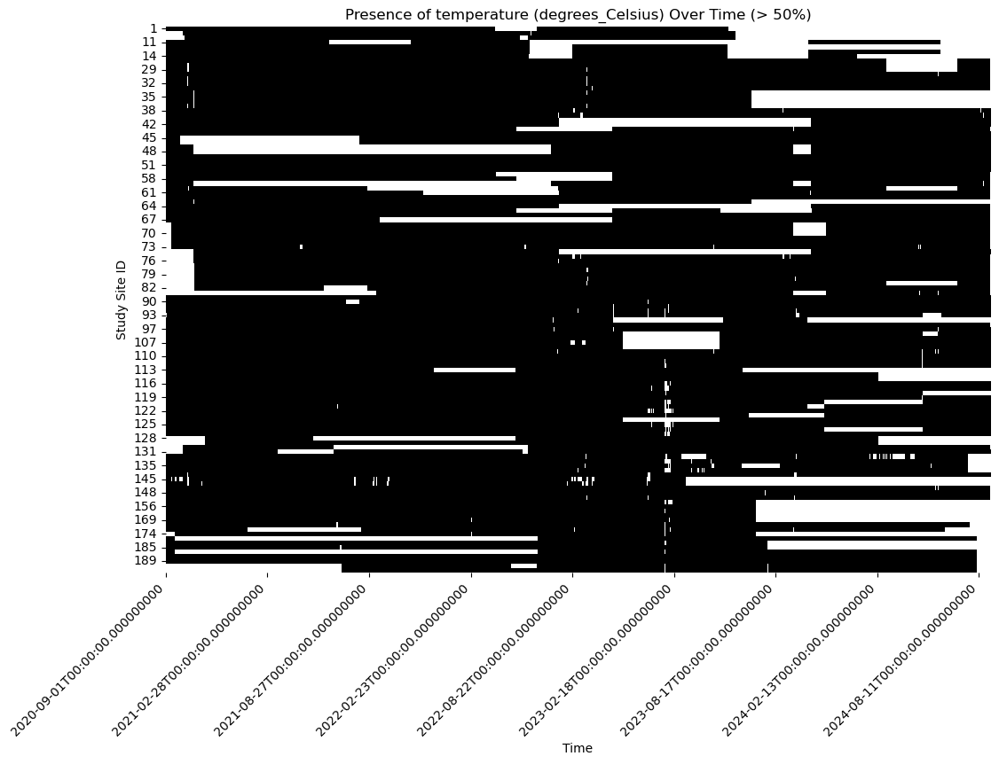
Our objective is to fill in the gaps in this dataset.

We save this dataset for subsequent analysis. While in this case study, the data happens to be temperature data the overall process should be applicable to any dataset in this form.

df_selected.to_csv('dataset.csv')

And let’s save the information about where each of those selected study sites.

study_sites_selected = study_sites.iloc[selected_sites]
study_sites_selected.to_csv('study_sites.csv')

import holoviews as hv
hv.extension('bokeh')

df_selected.columns = df_selected.columns.astype(str)

dictionary = {i: hv.Curve(df_selected[str(i)], 
                          label=f"{study_sites_selected.loc[i, 'waterbody']} - {study_sites_selected.loc[i, 'station']} ({study_sites_selected.loc[i, 'depth (m)']}m)")
                for i in study_sites_selected.index }
hv.HoloMap(dictionary, kdims='Study Site').opts(aspect=2)

Time Series Imputation for Oceanographic Data

CMAR Water Quality Datasets

Time Series Imputation for Oceanographic Data

Make missing gap