6. Case Study: CMAR Water Quality Data - Shelburne County - Time Series Imputation for Oceanographic Data

Download the Dataset¶

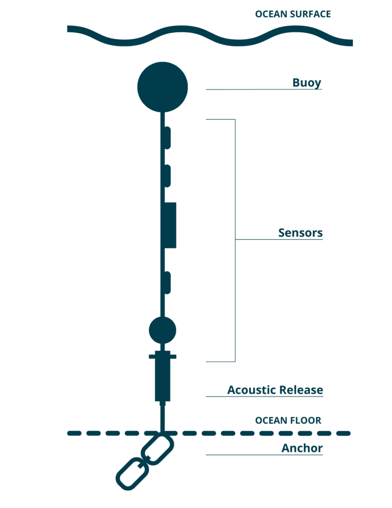
We want to analyze the Centre for Marine Applied Research (CMAR) Water Quality dataset. This dataset is comprised of various moorings with temperator sensors at fixed depths off the coast of Shelburne County in Nova Scotia.

from erddapy import ERDDAP
import os
import pandas as pd
import numpy as np

import panel as pn
import holoviews as hv
from holoviews import opts
hv.extension('bokeh')
pn.extension()

The data is available from CIOOS Atlantic via ERDDAP.

e = ERDDAP(
    server = "https://cioosatlantic.ca/erddap",
    protocol = "tabledap"
)

e.dataset_id = 'mq2k-54s4' # Shelburne County Water Quality Data

e.variables = [
 'waterbody',
 'station',
 'depth',
 'time',
 'temperature',
 'qc_flag_temperature']

allowed_stations = ['Ingomar', 'Blue Island', 'McNutts Island', 'Taylors Rock']

# only grab data from county with data within study period
e.constraints = {
    'station=~': '|'.join(allowed_stations),
    "time>=": "2018-05-15", 
    "time<=": "2022-05-14"
}

Download the data (caching locally so that we don’t have to download if this notebook is run again.)

%%time
os.makedirs('data', exist_ok=True)

csvfile = f"data/ShelburneCounty.csv.gz"

if not os.path.exists(csvfile):
    df = e.to_pandas()
    df.to_csv(csvfile, compression='gzip', index=False)

CPU times: user 43 μs, sys: 1 μs, total: 44 μs
Wall time: 44.6 μs

df = pd.read_csv(csvfile)

df.sample(10)

# Filter rows where QC flag is 'Pass'
df_filtered = df[df['qc_flag_temperature'] == 'Pass'].copy()

# Ensure time column is datetime and remove timezone
df_filtered['time (UTC)'] = pd.to_datetime(df_filtered['time (UTC)']).dt.tz_localize(None)

# Create a new column for date only (drop time component)
df_filtered['date'] = df_filtered['time (UTC)'].dt.date

# Group and aggregate
daily_avg = (
    df_filtered
    .groupby(['waterbody', 'station', 'depth (m)', 'date'])['temperature (degrees_Celsius)']
    .mean()
    .round(3)  # Limit to 3 decimal places
    .reset_index()
    .rename(columns={'temperature (degrees_Celsius)': 'daily_avg_temperature'})
)

# Pivot the data: rows = date, columns = station, values = daily average temperature
pivot_df = daily_avg.pivot_table(
    index='date',
    columns=['station', 'depth (m)'],
    values='daily_avg_temperature'
)

# Flatten MultiIndex columns into strings like "Blue Island @ 10.0m"
pivot_df.columns = [f"{station.replace(' ','')}_{depth:.0f}m" for station, depth in pivot_df.columns]

pivot_df

pivot_df.to_csv('dataset_shelburne.csv')

Visualize the series data¶

df = pd.read_csv('dataset_shelburne.csv', parse_dates=True, index_col=0)

# Create a dropdown selector
site_selector = pn.widgets.Select(name='Site', options=list(df.columns))

def highlight_nan_regions(label):

    series = df[label]
    
    # Identify NaN regions
    is_nan = series.isna()
    nan_ranges = []
    current_start = None

    for date, missing in is_nan.items():
        if missing and current_start is None:
            current_start = date
        elif not missing and current_start is not None:
            nan_ranges.append((current_start, date))
            current_start = None
    if current_start is not None:
        nan_ranges.append((current_start, series.index[-1]))

    # Create shaded regions
    spans = [
        hv.VSpan(start, end).opts(color='red', alpha=0.2)
        for start, end in nan_ranges
    ]

    curve = hv.Curve(series, label=label).opts(
        width=900, height=250, tools=['hover', 'box_zoom', 'pan', 'wheel_zoom'],
        show_grid=True, title=label
    )

    return curve * hv.Overlay(spans)
    
interactive_plot = hv.DynamicMap(pn.bind(highlight_nan_regions, site_selector))

pn.Column(site_selector, interactive_plot, 'Hightlights regions are gaps that need to imputed.')

Impute the gaps¶

We have determined that the MissForestappears to work reasonably well when imputing artificially large gaps.

We use it to gap fill the missing data in this dataset.

from imputeMF import imputeMF

df_imputed = pd.DataFrame(imputeMF(df.values, 10, print_stats=True), columns=df.columns, index=df.index)

df_imputed.to_csv('dataset_shelburne_imputed.csv')

Statistics:
iteration 1, gamma = 0.034447563594337524
Statistics:
iteration 2, gamma = 0.0005790595084971316
Statistics:
iteration 3, gamma = 7.028340599830522e-05
Statistics:
iteration 4, gamma = 2.5996539045398812e-05
Statistics:
iteration 5, gamma = 1.3475555988408412e-05
Statistics:
iteration 6, gamma = 1.3575497441166254e-05

def highlight_imputed_regions(label):

    series = df[label]
    series_imputed = df_imputed[label]
    
    # Identify NaN regions
    is_nan = series.isna()
    nan_ranges = []
    current_start = None

    for date, missing in is_nan.items():
        if missing and current_start is None:
            current_start = date
        elif not missing and current_start is not None:
            nan_ranges.append((current_start, date))
            current_start = None
    if current_start is not None:
        nan_ranges.append((current_start, series.index[-1]))

    # Create shaded regions
    spans = [
        hv.VSpan(start, end).opts(color='red', alpha=0.2)
        for start, end in nan_ranges
    ]

    curve = hv.Curve(series_imputed, label=label).opts(
        width=900, height=250, tools=['hover', 'box_zoom', 'pan', 'wheel_zoom'],
        show_grid=True, title=label
    )

    return curve * hv.Overlay(spans)
    
interactive_plot = hv.DynamicMap(pn.bind(highlight_imputed_regions, site_selector))

pn.Column(site_selector, interactive_plot)

Highlighted regions have been imputed using MissForest.