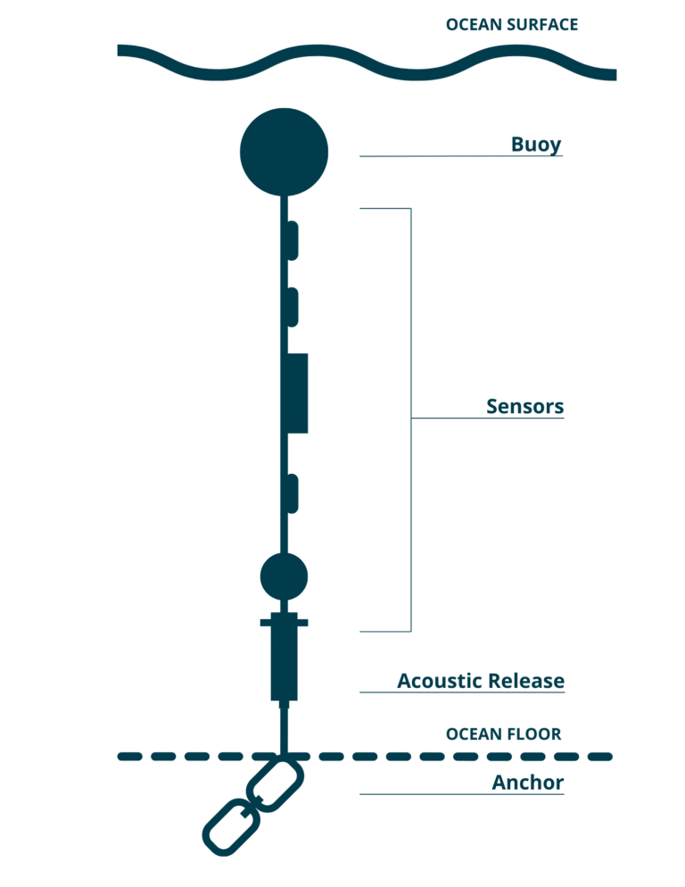
We want to analyze the Centre for Marine Applied Research (CMAR) Water Quality dataset. This dataset is comprised of various moorings with temperator sensors at fixed depths at many locations around Nova Scotia.

from erddapy import ERDDAP
import os
import pandas as pd
import numpy as np
import matplotlib.pyplot as plt
from tqdm import tqdm

import panel as pn
import holoviews as hv
from holoviews import opts
hv.extension('bokeh')
pn.extension()Download the Dataset
The data is available from CIOOS Atlantic
e = ERDDAP(
    server = "https://cioosatlantic.ca/erddap",
    protocol = "tabledap"
)
Determine the datasetID for each CMAR Water Quality dataset.
The study period is 2020-09-01 to 2024-08-31.
e.dataset_id = 'allDatasets'
e.variables = ['datasetID', 'institution', 'title', 'minTime', 'maxTime']

# only grab data from county with data within study period
e.constraints = {'maxTime>=': '2020-09-01', 'minTime<=': '2024-08-31'}
df_allDatasets = e.to_pandas()
df_CMAR_datasets = df_allDatasets[df_allDatasets['institution'].str.contains('CMAR') & df_allDatasets['title'].str.contains('Water Quality Data')].copy()
df_CMAR_datasets['county'] = df_CMAR_datasets['title'].str.removesuffix(' County Water Quality Data')
df_CMAR_datasetsFor each of these datasets, we download the temperature data locally.
e.variables = [
 'waterbody',
 'station',
 'deployment_start_date',
 'deployment_end_date',
 'time',
 'depth',
 'temperature',
 'qc_flag_temperature']

e.constraints = { "time>=": "2020-09-01", "time<=": "2024-08-31" }
This next step can takes 15+ minutes so we locally cache the data so it only has to be downloaded once.
%%time

os.makedirs('data', exist_ok=True)

for index, row in df_CMAR_datasets.iterrows():

    csvfile = f"data/{row['county']}.csv.gz"

    if os.path.exists(csvfile):
        continue

    print(f"Downloading {row['title']}...")
    e.dataset_id = row['datasetID']
    df = e.to_pandas()

    df.to_csv(csvfile, compression='gzip', index=False)
Downloading Shelburne County Water Quality Data...
CPU times: user 5.87 s, sys: 175 ms, total: 6.05 s
Wall time: 20.5 s
We now have the following .csv files stored locally:
!ls -lh data/total 129M
-rw-r--r-- 1 jmunroe jmunroe 1.4M Aug 15 09:07 Annapolis.csv.gz
-rw-r--r-- 1 jmunroe jmunroe 4.9M Aug 15 09:08 Antigonish.csv.gz
-rw-r--r-- 1 jmunroe jmunroe 1.3M Aug 15 09:08 Colchester.csv.gz
-rw-r--r-- 1 jmunroe jmunroe 5.7M Aug 15 09:09 Digby.csv.gz
-rw-r--r-- 1 jmunroe jmunroe 45M Aug 15 09:16 Guysborough.csv.gz
-rw-r--r-- 1 jmunroe jmunroe 7.9M Aug 15 09:18 Halifax.csv.gz
-rw-r--r-- 1 jmunroe jmunroe 1.5M Aug 15 09:18 Inverness.csv.gz
-rw-r--r-- 1 jmunroe jmunroe 17M Aug 15 09:21 Lunenburg.csv.gz
-rw-r--r-- 1 jmunroe jmunroe 2.0M Aug 15 09:22 Pictou.csv.gz
-rw-r--r-- 1 jmunroe jmunroe 2.9M Aug 15 09:23 Queens.csv.gz
-rw-r--r-- 1 jmunroe jmunroe 3.5M Aug 15 09:24 Richmond.csv.gz
-rw-r--r-- 1 jmunroe jmunroe 6.4M Oct 6 12:32 Shelburne.csv.gz
-rw-r--r-- 1 jmunroe jmunroe 15M Oct 5 22:28 ShelburneCounty.csv.gz
-rw-r--r-- 1 jmunroe jmunroe 8.1K Aug 15 09:25 Victoria.csv.gz
-rw-r--r-- 1 jmunroe jmunroe 8.3M Aug 15 09:28 Yarmouth.csv.gz
-rw-r--r-- 1 jmunroe jmunroe 6.8M Aug 15 11:26 ais_tempdata.csv.gz
Organize observations by physical location
We need to organize and sort the observations so that we are considering only the observation for a single sensor in temporal order.
This will remove all of the duplicated metadata within each .csv files.
os.makedirs('segments', exist_ok=True)

all_segment_metadata = []
for index, row in tqdm(list(df_CMAR_datasets.iterrows())):

    csvfile = f"data/{row['county']}.csv.gz"

    df = pd.read_csv(csvfile)

    df['deployment_start'] = df['deployment_start_date (UTC)'].str[:10]
    df['deployment_end'] = df['deployment_end_date (UTC)'].str[:10]
    df.drop(columns=['deployment_start_date (UTC)', 'deployment_end_date (UTC)'], inplace=True)

    df['segment'] = df[['waterbody', 'station', 'depth (m)',
                     'deployment_start', 'deployment_end',
                     ]].agg(lambda x: row['county'] + '_' + '_'.join([str(y) for y in x]), axis=1)

    df_metadata = df[['segment', 'waterbody', 'station', 'depth (m)',
                     'deployment_start', 'deployment_end',
                     ]]

    df_metadata = df_metadata.drop_duplicates()
    all_segment_metadata.append(df_metadata)

    df_data = df.drop(columns=['waterbody', 'station', 'depth (m)',
                                 'deployment_start', 'deployment_end',
                              ])

    df_data = df_data.sort_values(by=['segment', 'time (UTC)'])

    df_data.set_index(['segment', 'time (UTC)'], inplace=True)

    for key, segment_df in df_data.groupby(level=0):
        csvfile = f'segments/{key}.csv'
        segment_df = segment_df.droplevel(0)
        segment_df.to_csv(csvfile)

df_metadata = pd.concat(all_segment_metadata)
df_metadata.set_index('segment', inplace=True)
df_metadata.to_csv('metadata.csv')
100%|███████████████████████████████████████████████████████████████████████████████████| 14/14 [02:09<00:00, 9.28s/it]
!ls -lh segments/ | wc 1082 12409 126443
We have 1082 distinct observational time series taken at various locations and depths around Nova Scotia during the period of 2020-09-01 to 2024-08-31
df_metadata.sample(8)Combine Time Series and Downsample
df_metadata = pd.read_csv('metadata.csv')Sensors are deployed many different depths in the water column.
df_metadata['depth (m)'].unique()array([ 2. , 6. , 4. , 1. , 1.3 , 0.5 , 1.5 , 0.4 , 0.8 ,
1.6 , 16. , 15. , 14. , 0. , 5. , 7. , 30. , 18. ,
10. , 20. , 3. , 3.5 , 0.41, 26. , 25. , 75. , 40. ,
50. , 22. , 28. , 36. , 9. , 60. , 44. , 24. , 27. ,
12. , 21. , 16.5 , 8. , 17.5 , 37. , 11. , 13. , 4.5 ])Most often, there are standard depths that are most often used:
df_metadata['depth (m)'].value_counts().head(15)depth (m)
2.0 195
5.0 184
10.0 156
15.0 132
20.0 93
1.0 50
30.0 35
25.0 25
0.5 18
40.0 16
4.0 14
3.0 13
1.5 10
8.0 10
27.0 10
Name: count, dtype: int64Let’s group these observation segments into more limited number of study sites where the waterbody, station, and depth are the same even if the sensor itself is replaced.
depths_list = [2.0, 5.0, 10.0, 15.0, 20.0]
study_sites = df_metadata[df_metadata['depth (m)'].isin(depths_list)][['waterbody', 'station', 'depth (m)']].drop_duplicates()
study_sites.reset_index(drop=True, inplace=True)study_sitesFor any of these study sites we can consider all of the observational segements at that station and depth. For example, consider one study site that represents four distinct observational sequences:
study_site = study_sites.iloc[37]

subset = df_metadata[ (df_metadata['waterbody'] == study_site['waterbody']) &  (df_metadata['station'] == study_site['station']) & (df_metadata['depth (m)'] == study_site['depth (m)'])]
display(subset)

fig, ax = plt.subplots(2,1, figsize=(12,6),sharex=True)

variable = 'temperature (degrees_Celsius)'
qc_flag = 'qc_flag_temperature'

series_segments = []
for index, row in subset.iterrows():

    csvfile = f"segments/{row['segment']}.csv"

    series = pd.read_csv(csvfile, index_col='time (UTC)', parse_dates=True)
    series.sort_index(inplace=True)

    # blank out observations that do not pass QC
    series[series[qc_flag] != 'Pass'] = np.nan
    series = series.drop(columns=[qc_flag])

    ax[0].plot(series.index, series[variable])

    ax[0].set_ylabel(variable)
    ax[0].set_title(f'{study_site.waterbody}:{study_site.station} at {study_site["depth (m)"]} m')

    if series.count()[variable] > 0:
        series_segments.append(series)

series_df = pd.concat(series_segments)
series_df.sort_index(inplace=True)

ax[1].set_title('Resampled to daily mean')
daily_series_df = series_df.resample('D').min()
ax[1].plot(daily_series_df.index, daily_series_df[variable], label='min', linewidth=0.5)
daily_series_df = series_df.resample('D').max()
ax[1].plot(daily_series_df.index, daily_series_df[variable], label='max', linewidth=0.5)
daily_series_df = series_df.resample('D').mean()
ax[1].plot(daily_series_df.index, daily_series_df[variable], label='mean')

ax[1].set_ylabel(variable)

plt.show()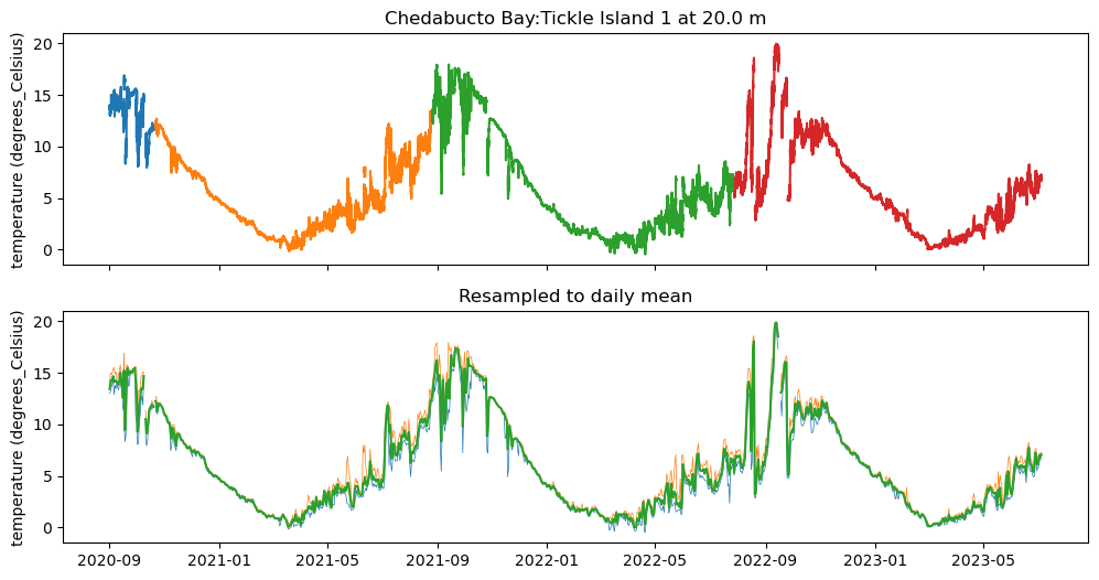
At the time scale of four years, daily means are sufficient to see the cycle. The plot above shows the daily minimum and daily maximum.
Combine segments into time series
We aggregate together these different segments from different deployments (and possibly different sensor) to create a complete daily time series at each station and depth in our study area:
start_date = "2020-09-01"
end_date = "2024-08-31"

daily_time_index = pd.date_range(start=start_date, end=end_date, freq='D')

all_timeseries = []

for study_site_id in tqdm(study_sites.index):

    study_site = study_sites.iloc[study_site_id]
    #print(f'[{study_site_id}] {study_site.waterbody}:{study_site.station} at {study_site['depth (m)']} m')
    study_site_name = f"{study_site.waterbody.replace(' ','')}_{study_site.station.replace(' ','')}_{study_site['depth (m)']:.0f}"

    subset = df_metadata[ (df_metadata['waterbody'] == study_site['waterbody']) &  (df_metadata['station'] == study_site['station']) & (df_metadata['depth (m)'] == study_site['depth (m)'])].copy()

    segments = []
    for segment_id, row in subset.iterrows():

        csvfile = f"segments/{row['segment']}.csv"
        segment = pd.read_csv(csvfile, index_col='time (UTC)', parse_dates=True)

        segment.sort_index(inplace=True)

        # blank out observations that do not pass QC
        segment[segment[qc_flag] != 'Pass'] = np.nan
        segment = segment.drop(columns=[qc_flag])

        if segment.count()[variable] > 0:
            segments.append(segment)

    if len(segments) > 0:

        timeseries = pd.concat(segments)
        timeseries.columns = [study_site_id]

        timeseries.sort_index(inplace=True)

        daily_timeseries = timeseries.resample('D').mean()

        all_timeseries.append(daily_timeseries)

dataset = pd.concat(all_timeseries, axis=1)
100%|█████████████████████████████████████████████████████████████████████████████████| 201/201 [00:27<00:00, 7.21it/s]
This is our temperature dataset. It also define the starting point for reproducing this analysis with a different data set. We have measurements on same time resolution for many different measurements. Each column in the dataset represents a different measurement. We use NaN to represent daily measurements that are missing.
The goal of imputation is to make a good estimate of what values to replace those NaN that, while still an estimate, are justifiable.
dataset.sample(10)We save this dataset for subsequent analysis. For this notebook series, any dataset in this form could be used for the subsequent steps in the analysis.
dataset.to_csv('dataset_cmar.csv')We also save the list of study sites to be able to map back the numerical study_id to a physical location.
study_sites.to_csv('study_sites.csv')Explore
df = pd.read_csv('dataset_cmar.csv', parse_dates=True, index_col=0)This dataset covers four years of daily observations (2020-09-01 to 2024-08-31) for 201 different “sites” (different stations and vertical depths).
Missing Data
How much of this dataset is actually missing?
non_missing_data = ~df.isna()

import seaborn as sns
from matplotlib.dates import DateFormatter

plt.figure()
sns.heatmap(non_missing_data.T, xticklabels= 180, cmap=['white', 'black'], cbar=False)

plt.ylabel('Study Site ID')
plt.title(f'Presence of measurement over time')

# Rotating the time axis labels for better readability
plt.xticks(rotation=45, ha='right')

plt.show()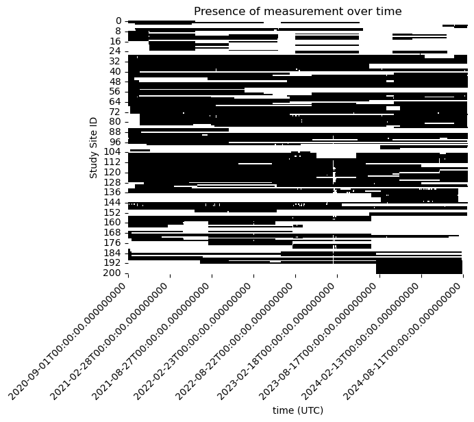
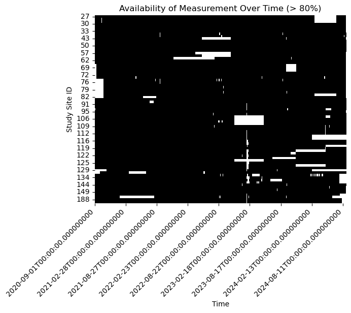
Some of our study site have very limited measurements at any time. We focus the problem more narrowly and ask what is the best estimate of the missing data when there is at least 50% of the observations available at a study site.
# Calculate the percentage of non-missing data for each study site
non_missing_percentage = df.notna().mean() * 100

# Filter study sites with at least 50% non-missing data
selected_sites = non_missing_percentage[non_missing_percentage >= 80].index
df = df[selected_sites]
# Creating a boolean DataFrame where True indicates non-missing data
non_missing_data = ~df.isna()
# Plotting
plt.figure()
sns.heatmap(non_missing_data.T, xticklabels= 180, cmap=['white', 'black'], cbar=False)
# Formatting the time axis labels
date_format = DateFormatter('%Y-%m-%d %H:%M')
#plt.gca().xaxis.set_major_formatter(date_format)
plt.xlabel('Time')
plt.ylabel('Study Site ID')
plt.title(f'Availability of Measurement Over Time (> 80%)')
# Rotating the time axis labels for better readability
plt.xticks(rotation=45, ha='right')
plt.show()
Our objective is to fill in the gaps in this dataset.
# Create a dropdown selector
site_selector = pn.widgets.Select(name='Site', options=list(df.columns))

def highlight_nan_regions(label):

    series = df[label]

    # Identify NaN regions
    is_nan = series.isna()
    nan_ranges = []
    current_start = None

    for date, missing in is_nan.items():
        if missing and current_start is None:
            current_start = date
        elif not missing and current_start is not None:
            nan_ranges.append((current_start, date))
            current_start = None
    if current_start is not None:
        nan_ranges.append((current_start, series.index[-1]))

    # Create shaded regions
    spans = [
        hv.VSpan(start, end).opts(color='red', alpha=0.2)
        for start, end in nan_ranges
    ]

    curve = hv.Curve(series, label=label).opts(
        width=900, height=250, tools=['hover', 'box_zoom', 'pan', 'wheel_zoom'],
        show_grid=True, title=label
    )

    return curve * hv.Overlay(spans)

interactive_plot = hv.DynamicMap(pn.bind(highlight_nan_regions, site_selector))

pn.Column(site_selector, interactive_plot, 'Hightlights regions are gaps that need to imputed.')study_sites = pd.read_csv('study_sites.csv')Impute
from imputeMF import imputeMFdf_imputed = pd.DataFrame(imputeMF(df.values, 10, print_stats=True), columns=df.columns, index=df.index)Statistics:
iteration 1, gamma = 0.00967529305597932
Statistics:
iteration 2, gamma = 0.0006342440790753214
Statistics:
iteration 3, gamma = 6.861681732348203e-05
Statistics:
iteration 4, gamma = 3.260598973974818e-05
Statistics:
iteration 5, gamma = 1.280284588659504e-05
Statistics:
iteration 6, gamma = 1.3532914597853127e-05
df_imputed.to_csv('dataset_cmar_imputed.csv')def highlight_imputed_regions(label):
series = df[label]
series_imputed = df_imputed[label]
# Identify NaN regions
is_nan = series.isna()
nan_ranges = []
current_start = None
for date, missing in is_nan.items():
if missing and current_start is None:
current_start = date
elif not missing and current_start is not None:
nan_ranges.append((current_start, date))
current_start = None
if current_start is not None:
nan_ranges.append((current_start, series.index[-1]))
# Create shaded regions
spans = [
hv.VSpan(start, end).opts(color='red', alpha=0.2)
for start, end in nan_ranges
]
curve = hv.Curve(series_imputed, label=label).opts(
width=900, height=250, tools=['hover', 'box_zoom', 'pan', 'wheel_zoom'],
show_grid=True, title=label
)
return curve * hv.Overlay(spans)
interactive_plot = hv.DynamicMap(pn.bind(highlight_imputed_regions, site_selector))
pn.Column(site_selector, interactive_plot)